---
engine: knitr
---
# Results
```{r}
#| label: setup-results
#| code-summary: "Setup and libraries"
#| code-fold: true
#| message: false
#| warning: false
source("setup_params.R")

library("tidyverse")
library("janitor")
library("stringr")
library("here")
library("knitr")
library("kableExtra")
library("ggrepel")
library("scales")
library("jsonlite")
library("purrr")
library("tibble")

# Theme and colors — crisp palette (high saturation, maximum separation)
UJ_ORANGE <- "#E8722A"   # vivid saffron orange
UJ_GREEN  <- "#2D9D5E"   # rich emerald green
UJ_BLUE   <- "#2B7CE9"   # clear azure blue

MODEL_COLORS <- c(
  "GPT-5 Pro"        = "#E8722A",   # saffron orange (focal)
  "GPT-5.2 Pro"      = "#D62839",   # bright crimson
  "GPT-4o-mini"      = "#17B890",   # vivid teal
  "Claude Sonnet 4"  = "#A855F7",   # vivid purple
  "Claude Opus 4.6"  = "#7C3AED",   # deep violet
  "Gemini 2.0 Flash" = "#2B7CE9",   # clear azure
  "Human"            = "#2D9D5E"    # emerald green
)

theme_uj <- function(base_size = 12) {
  theme_minimal(base_size = base_size) +
    theme(
      panel.grid.minor   = element_blank(),
      panel.grid.major   = element_line(linewidth = 0.3, color = "grey88"),
      plot.title          = element_text(face = "bold", size = rel(1.1)),
      plot.title.position = "plot",
      plot.subtitle       = element_text(color = "grey40", size = rel(0.9)),
      plot.caption        = element_text(color = "grey50", size = rel(0.8), hjust = 0),
      axis.title          = element_text(size = rel(0.95)),
      axis.text           = element_text(size = rel(0.88)),
      legend.position     = "bottom",
      legend.text         = element_text(size = rel(0.88)),
      legend.title        = element_text(size = rel(0.9), face = "bold"),
      strip.text          = element_text(face = "bold", size = rel(0.95))
    )
}

canon_metric <- function(x) dplyr::recode(
  x,
  "advancing_knowledge" = "adv_knowledge",
  "open_science"        = "open_sci",
  "logic_communication" = "logic_comms",
  "global_relevance"    = "gp_relevance",
  "claims_evidence"     = "claims",
  .default = x
)

`%||%` <- function(x, y) if (!is.null(x)) x else y
```
```{r}
#| label: load-human-data-results
#| code-fold: true
#| code-summary: "Load human evaluation data"
#| message: false
UJmap <- read_delim("data/UJ_map.csv", delim = ";", show_col_types = FALSE) |>
  mutate(label_paper_title = research, label_paper = paper) |>
  select(c("label_paper_title", "label_paper"))

rsx <- read_csv("data/rsx_evalr_rating.csv", show_col_types = FALSE) |>
  clean_names() |>
  mutate(label_paper_title = research) |>
  select(-c("research"))

research <- read_csv("data/research.csv", show_col_types = FALSE) |>
  clean_names() |>
  filter(status == "50_published evaluations (on PubPub, by Unjournal)") |>
  left_join(UJmap, by = c("label_paper_title")) |>
  mutate(doi = str_trim(doi)) |>
  mutate(label_paper = case_when(
    doi == "https://doi.org/10.3386/w31162" ~ "Walker et al. 2023",
    doi == "doi.org/10.3386/w32728" ~ "Hahn et al. 2025",
    doi == "https://doi.org/10.3386/w30011" ~ "Bhat et al. 2022",
    doi == "10.1093/wbro/lkae010" ~ "Crawfurd et al. 2023",
    TRUE ~ label_paper
  )) |>
  left_join(rsx, by = c("label_paper_title"))

key_map <- research |>
  transmute(label_paper_title = str_trim(label_paper_title), label_paper = label_paper) |>
  filter(!is.na(label_paper_title)) |>
  distinct(label_paper_title, label_paper) |>
  group_by(label_paper_title) |>
  slice(1) |>
  ungroup()

rsx_research <- rsx |>
  mutate(label_paper_title = str_trim(label_paper_title)) |>
  left_join(key_map, by = "label_paper_title", relationship = "many-to-one")

metrics_human <- rsx_research |>
  mutate(criteria = canon_metric(criteria)) |>
  filter(criteria %in% c("overall", "claims", "methods", "adv_knowledge", "logic_comms", "open_sci", "gp_relevance")) |>
  transmute(
    paper = label_paper, criteria, evaluator, model = "Human",
    mid = as.numeric(middle_rating),
    lo = suppressWarnings(as.numeric(lower_ci)),
    hi = suppressWarnings(as.numeric(upper_ci))
  ) |>
  filter(!is.na(paper), !is.na(mid)) |>
  mutate(
    lo = ifelse(is.finite(lo), pmax(0, pmin(100, lo)), NA_real_),
    hi = ifelse(is.finite(hi), pmax(0, pmin(100, hi)), NA_real_)
  ) |>
  mutate(across(c(mid, lo, hi), ~ round(.x, 4))) |>
  distinct(paper, criteria, model, evaluator, mid, lo, hi)

human_avg <- metrics_human |>
  filter(criteria == "overall") |>
  group_by(paper) |>
  summarise(
    human_mid = mean(mid, na.rm = TRUE),
    human_lo = mean(lo, na.rm = TRUE),
    human_hi = mean(hi, na.rm = TRUE),
    n_human = n(),
    .groups = "drop"
  )

n_human_papers <- n_distinct(metrics_human$paper)
n_human_evaluators <- n_distinct(metrics_human$evaluator)
```
```{r}
#| label: load-llm-data-results
#| code-fold: true
#| code-summary: "Load LLM evaluation data (all models)"
#| message: false
model_dirs <- list(
  "gpt5_pro_updated_jan2026" = "GPT-5 Pro",
  "gpt52_pro_focal_jan2026" = "GPT-5.2 Pro",
  "gpt_4o_mini_2024_07_18" = "GPT-4o-mini",
  "claude_sonnet_4_20250514" = "Claude Sonnet 4",
  "claude_opus_4_6" = "Claude Opus 4.6",
  "gemini_2.0_flash" = "Gemini 2.0 Flash"
)

parse_response <- function(path, model_name) {
  tryCatch({
    r <- jsonlite::fromJSON(path, simplifyVector = FALSE)
    paper <- basename(path) |>
      str_replace("\\.response\\.json$", "") |>
      str_replace_all("_", " ")

    parsed <- NULL
    if (!is.null(r$parsed) && length(r$parsed) > 0) {
      parsed <- r$parsed
    } else if (!is.null(r$output_text) && nchar(r$output_text) > 0) {
      txt <- r$output_text
      txt <- sub("^\\s*```[a-z]*\\s*\n?", "", txt)
      txt <- sub("\\s*```\\s*$", "", txt)
      parsed <- jsonlite::fromJSON(txt, simplifyVector = TRUE)
    } else if (!is.null(r$output)) {
      msg <- purrr::detect(r$output, ~ .x$type == "message", .default = NULL)
      if (!is.null(msg) && length(msg$content) > 0) {
        parsed <- jsonlite::fromJSON(msg$content[[1]]$text, simplifyVector = TRUE)
      }
    }

    if (is.null(parsed)) return(NULL)

    metrics <- parsed$metrics
    metric_rows <- list()
    tier_rows <- list()
    tier_names <- c("tier_should", "tier_will", "journal_should", "journal_will")

    for (nm in names(metrics)) {
      if (nm %in% tier_names) {
        tier_kind <- sub("^journal_", "tier_", nm)
        tier_rows[[length(tier_rows) + 1]] <- tibble(
          paper = paper, model = model_name, tier_kind = tier_kind,
          score = metrics[[nm]]$score,
          ci_lower = metrics[[nm]]$ci_lower,
          ci_upper = metrics[[nm]]$ci_upper
        )
      } else {
        metric_rows[[length(metric_rows) + 1]] <- tibble(
          paper = paper, model = model_name, metric = nm,
          midpoint = metrics[[nm]]$midpoint,
          lower_bound = metrics[[nm]]$lower_bound,
          upper_bound = metrics[[nm]]$upper_bound
        )
      }
    }

    input_tok <- r$usage$input_tokens %||% r$input_tokens
    output_tok <- r$usage$output_tokens %||% r$output_tokens

    list(
      metrics = bind_rows(metric_rows),
      tiers = bind_rows(tier_rows),
      tokens = tibble(
        paper = paper, model = model_name,
        input_tokens = input_tok %||% NA_integer_,
        output_tokens = output_tok %||% NA_integer_
      )
    )
  }, error = function(e) NULL)
}

load_all_llm <- function() {
  all_metrics <- list()
  all_tiers <- list()
  all_tokens <- list()

  for (dir_name in names(model_dirs)) {
    model_name <- model_dirs[[dir_name]]
    json_dir <- here("results", dir_name, "json")

    if (dir.exists(json_dir)) {
      files <- list.files(json_dir, pattern = "\\.response\\.json$", full.names = TRUE)

      for (f in files) {
        result <- parse_response(f, model_name)
        if (!is.null(result)) {
          all_metrics[[length(all_metrics) + 1]] <- result$metrics
          all_tiers[[length(all_tiers) + 1]] <- result$tiers
          all_tokens[[length(all_tokens) + 1]] <- result$tokens
        }
      }
    }
  }

  list(
    metrics = bind_rows(all_metrics) |> mutate(criteria = canon_metric(metric)),
    tiers = bind_rows(all_tiers),
    tokens = bind_rows(all_tokens)
  )
}

llm_data <- load_all_llm()
llm_metrics <- llm_data$metrics
llm_tiers <- llm_data$tiers
llm_tokens <- llm_data$tokens

# Reconcile LLM filenames with human labels for papers where the citation year
# differs but the manuscript is the same (verified by title/DOI/content):
#  - "Trammel and Aschenbrenner 2024" (file) == human "Existential risk and
#     growth" == UJ label "Trammel and Aschenbrenner 2025"
#  - "Liang et al 2023" (file) == human "The Environmental Effects of Economic
#     Production" == UJ label "Liang et al. 2021"
# (LLM file "Liang et al. 2025" is a different paper — China SMC — left as is.)
canon_paper <- function(x) dplyr::recode(
  x,
  "Trammel and Aschenbrenner 2024" = "Trammel and Aschenbrenner 2025",
  "Liang et al 2023"               = "Liang et al. 2021",
  .default = x
)
llm_metrics <- llm_metrics |> mutate(paper = canon_paper(paper))
llm_tiers   <- llm_tiers   |> mutate(paper = canon_paper(paper))
llm_tokens  <- llm_tokens  |> mutate(paper = canon_paper(paper))

n_llm_models <- n_distinct(llm_metrics$model)
n_llm_papers <- n_distinct(llm_metrics$paper)

matched_papers <- intersect(
  unique(metrics_human$paper),
  unique(llm_metrics$paper)
)
n_matched <- length(matched_papers)

# Focal sample: papers evaluated by GPT-5 Pro AND humans
focal_papers <- intersect(
  llm_metrics |> filter(model == "GPT-5 Pro") |> pull(paper) |> unique(),
  unique(metrics_human$paper)
)
n_focal <- length(focal_papers)

primary_model <- if ("GPT-5 Pro" %in% unique(llm_metrics$model)) "GPT-5 Pro" else unique(llm_metrics$model)[1]
```
```{r}
#| label: compute-hh-baseline
#| include: false
# Human-Human pairwise agreement (baseline for agreement tables).
# For papers with ≥2 evaluators, assign E1/E2 by row order within paper,
# then compute pairwise correlation and error metrics across all such papers.
hh_pairs <- metrics_human |>
filter(criteria == "overall", paper %in% focal_papers) |>
select(paper, evaluator, mid) |>
distinct() |>
group_by(paper) |>
filter(n() >= 2) |>
mutate(slot = paste0("E", row_number())) |>
ungroup() |>
pivot_wider(names_from = slot, values_from = c(mid, evaluator)) |>
filter(!is.na(mid_E1), !is.na(mid_E2))
hh_n <- nrow(hh_pairs)
hh_pearson <- round(cor(hh_pairs$mid_E1, hh_pairs$mid_E2), 3)
hh_spearman <- round(cor(hh_pairs$mid_E1, hh_pairs$mid_E2, method = "spearman"), 3)
hh_mae <- round(mean(abs(hh_pairs$mid_E1 - hh_pairs$mid_E2), na.rm = TRUE), 1)
hh_rmse <- round(sqrt(mean((hh_pairs$mid_E1 - hh_pairs$mid_E2)^2, na.rm = TRUE)), 1)
hh_bias <- sprintf("%+.1f", mean(hh_pairs$mid_E1 - hh_pairs$mid_E2, na.rm = TRUE))
hh_baseline_row <- tibble(
Model = "Human\u2013Human",
N = hh_n,
`Spearman ρ` = hh_spearman,
`Pearson r` = hh_pearson,
`Mean bias` = hh_bias,
RMSE = hh_rmse,
MAE = hh_mae
)
# Spearman-Brown correction factor (same logic as Appendix A).
# GPT-5 Pro rho is computed against the k-rater human mean; rho_HH compares
# individual raters. Multiply raw rho_HL by sb_factor for a fair comparison.
k_raters <- metrics_human |>
filter(criteria == "overall", paper %in% focal_papers) |>
group_by(paper) |>
summarise(k = n_distinct(evaluator), .groups = "drop") |>
summarise(k = mean(k)) |>
pull(k)
r_kk <- k_raters * hh_spearman / (1 + (k_raters - 1) * hh_spearman)
sb_factor <- sqrt(hh_spearman / r_kk)
spearman_ci95 <- function(rho, n) {
if (is.na(rho) || n < 4) return("—")
z <- atanh(rho)
se <- 1 / sqrt(n - 3)
sprintf("[%.2f, %.2f]", tanh(z - 1.96 * se), tanh(z + 1.96 * se))
}
```
```{r}
#| label: compute-bootstrap-ci
#| include: false
# Paired bootstrap over papers, on the same matched group as the H-H baseline
# (papers with >=2 human raters). Each draw resamples papers with replacement,
# recomputes (a) GPT-5 Pro vs human-mean Spearman rho with that draw's own
# Spearman-Brown correction and (b) pooled human-human pairwise rho, so the
# adjusted difference is evaluated on matched resamples. Draws where the
# human-human correlation is non-positive leave the correction undefined and
# are dropped.
set.seed(42)
B <- 2000
llm_overall_boot <- llm_metrics |>
filter(criteria == "overall", model == "GPT-5 Pro", paper %in% hh_pairs$paper) |>
inner_join(human_avg |> select(paper, human_mid), by = "paper") |>
select(paper, midpoint, human_mid)
boot_draws <- replicate(B, {
bp <- sample(llm_overall_boot$paper, replace = TRUE)
d_llm <- llm_overall_boot[match(bp, llm_overall_boot$paper), ]
r_llm <- suppressWarnings(cor(d_llm$human_mid, d_llm$midpoint,
method = "spearman", use = "complete.obs"))
d_hh <- hh_pairs[match(bp, hh_pairs$paper), ]
d_hh <- d_hh[!is.na(d_hh$mid_E1) & !is.na(d_hh$mid_E2), ]
r_hh <- if (nrow(d_hh) >= 5) {
suppressWarnings(cor(d_hh$mid_E1, d_hh$mid_E2,
method = "spearman", use = "complete.obs"))
} else NA_real_
r_adj <- if (!is.na(r_hh) && r_hh > 0) {
r_kk_d <- k_raters * r_hh / (1 + (k_raters - 1) * r_hh)
r_llm * sqrt(r_hh / r_kk_d)
} else NA_real_
c(r_llm = r_llm, r_hh = r_hh, r_adj = r_adj)
})
boot_ci_llm <- quantile(boot_draws["r_llm", ], c(0.025, 0.975), na.rm = TRUE)
boot_ci_hh <- quantile(boot_draws["r_hh", ], c(0.025, 0.975), na.rm = TRUE)
boot_diff <- boot_draws["r_adj", ] - boot_draws["r_hh", ]
boot_ci_diff <- quantile(boot_diff, c(0.025, 0.975), na.rm = TRUE)
boot_n_valid <- sum(!is.na(boot_diff))
fmt_ci <- function(ci) sprintf("[%.2f, %.2f]", ci[1], ci[2])
# Table captions built as strings so numbers resolve in every output format
# (inline `r` inside tbl-cap YAML is not evaluated in the PDF pass).
# ASCII only: non-ASCII characters in chunk-option strings get serialized as
# literal <U+XXXX> placeholders in the book PDF pass.
cap_tbl_model_agreement <- paste0(
"GPT-5 Pro overall-rating agreement. **Primary (matched) group**: same ", hh_n,
" papers as the H-H baseline (papers with at least 2 human raters). ",
"**Secondary group**: all ", n_focal,
" matched papers. **Spearman rho column**: the H-H row shows individual-vs-individual ",
"rank correlation (the reference, already on the natural scale); GPT-5 Pro rows show ",
"correlation vs. the human mean, which is upward-biased relative to H-H. ",
"**rho adj.**: Spearman-Brown corrected to the individual-rater equivalent (factor ",
sprintf("%.2f", sb_factor),
"), making GPT-5 Pro rows directly comparable to H-H. **95% CI**: Fisher-z. ",
"Bias = LLM minus Human. Full six-model comparison in [Appendix A](results_ratings.qmd)."
)
cap_tbl_criteria_agreement <- paste0(
"GPT-5 Pro agreement with human mean by criterion (N = ", n_focal,
" papers; N = ", hh_n, " for H-H). **H-H rho**: pairwise human evaluator rank ",
"correlation (reference; computed on ", hh_n, " papers with at least 2 raters; raw ",
"LLM rho is upward-biased vs. H-H rho, see @tbl-model-agreement-main). Positive bias ",
"= GPT-5 Pro rates higher on average. Note the variation across criteria: human ",
"evaluators agree strongly on some dimensions and barely at all on others ",
"(Open Science), setting expectations for LLM performance."
)
```
We evaluate GPT-5 Pro against human expert reviews from [The Unjournal](https://unjournal.pubpub.org) on `r n_focal` matched papers (papers with both GPT-5 Pro and human evaluations). The model receives the same PDF, system prompt mirroring The Unjournal rubric, and JSON schema requiring a diagnostic summary plus numeric midpoints and 90% credible intervals for every metric. Results for five additional models are reported in [Appendix A](results_ratings.qmd). Full methodological details appear in [Methods](methods.qmd).
We do not treat human ratings as ground truth. Quantitative percentile scoring is genuinely difficult: even domain experts disagree, and individual scores reflect both signal about paper quality and idiosyncratic tendencies (severity, topic familiarity, interpretation of the scale). Our question is whether an LLM provides signal *comparable to an additional expert rater*. The Human–Human baseline row in @tbl-model-agreement-main provides this reference. **Caution**: the LLM's *ρ* is computed against the *mean* of `r round(k_raters, 1)` human raters, which reduces noise and inflates apparent agreement relative to the individual-vs-individual ρ_HH. The Spearman-Brown adjusted column corrects for this; the fair comparison is ρ adj. vs. ρ_HH. Krippendorff's α~HH~ in the [human-baseline table in Appendix A](results_ratings.qmd) provides the criterion-level reference.
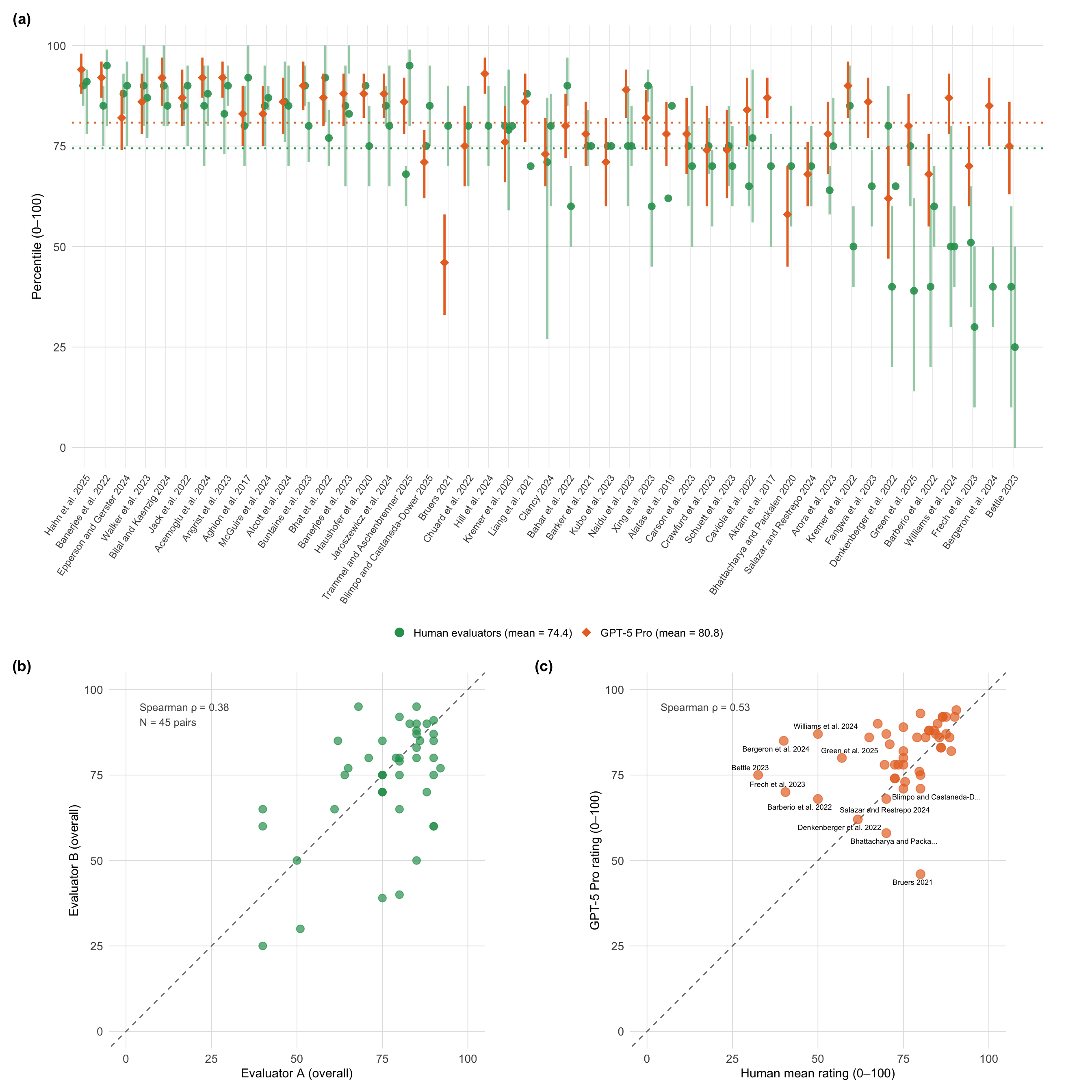
**Per-paper overview.** @fig-overview-combined presents three complementary views of overall (0--100 percentile) ratings. Panel (a) displays individual human evaluator ratings alongside GPT-5 Pro (orange diamonds) for each paper, revealing inter-rater variability---the self-reported 90% credible intervals from individual evaluators often span 20--40 percentile points. In most cases the LLM falls within the range of human opinions, though several papers show substantial divergence. Panel (b) plots all pairwise human evaluator combinations, making the human-human agreement ceiling directly visible. Panel (c) compares GPT-5 Pro ratings against human mean ratings with per-paper labels.
```{r}
#| label: fig-overview-combined
#| fig-cap: "Per-paper overall ratings (0--100 percentile). **(a)** Individual human evaluator midpoints (green circles) with each evaluator's self-reported 90% credible interval (reflecting their own uncertainty about the true score; the vertical separation between green dots per paper reflects inter-rater disagreement) and GPT-5 Pro (orange diamonds with CI), sorted by descending human mean. Dotted horizontal lines show grand means. **(b)** Pairwise human evaluator agreement: each point is one evaluator pair (papers with 3 raters contribute 3 points). **(c)** Human mean vs GPT-5 Pro overall rating; dashed diagonal is the identity line. Compare panels (b) and (c) directly to see whether LLM-human scatter is tighter than human-human scatter."
#| fig-width: 14
#| fig-height: 14
#| code-fold: true
library("patchwork")

# ── Panel (a): Forest plot ──
H_ind <- metrics_human |>
  filter(criteria == "overall", paper %in% matched_papers) |>
  mutate(
    lo = ifelse(is.finite(lo), pmax(0, lo), NA_real_),
    hi = ifelse(is.finite(hi), pmin(100, hi), NA_real_)
  )

ord <- H_ind |>
  group_by(paper) |>
  summarise(h_mean = mean(mid, na.rm = TRUE), .groups = "drop") |>
  arrange(desc(h_mean)) |>
  mutate(pos = row_number())

H_plot <- H_ind |>
  inner_join(ord, by = "paper") |>
  group_by(paper) |>
  mutate(
    off = (row_number() - (n() + 1) / 2) * 0.18,
    x   = pos + off
  ) |>
  ungroup()

L_c <- llm_metrics |>
  filter(criteria == "overall", model == primary_model, paper %in% matched_papers) |>
  group_by(paper) |>
  summarise(
    mid = mean(midpoint, na.rm = TRUE),
    lo  = suppressWarnings(min(coalesce(lower_bound, midpoint), na.rm = TRUE)),
    hi  = suppressWarnings(max(coalesce(upper_bound, midpoint), na.rm = TRUE)),
    .groups = "drop"
  ) |>
  inner_join(ord, by = "paper") |>
  mutate(x = pos - 0.18)

hbar     <- mean(ord$h_mean, na.rm = TRUE)
lbar     <- mean(L_c$mid, na.rm = TRUE)

# Legend labels embed grand means so the annotation text can be dropped
lbl_human <- sprintf("Human evaluators (mean = %.1f)", hbar)
lbl_gpt   <- sprintf("GPT-5 Pro (mean = %.1f)", lbar)

leg_colors <- setNames(c(UJ_GREEN, UJ_ORANGE),
                       c(lbl_human, lbl_gpt))
leg_shapes <- setNames(c(16L, 18L),
                       c(lbl_human, lbl_gpt))

p_forest <- if (nrow(L_c) > 0) {
  ggplot() +
    geom_vline(data = ord, aes(xintercept = pos), color = "grey92", linewidth = 0.3) +
    geom_hline(yintercept = hbar,      color = UJ_GREEN,    linetype = "dotted", linewidth = 0.8) +
    geom_hline(yintercept = lbar,      color = UJ_ORANGE,   linetype = "dotted", linewidth = 0.8) +
    geom_errorbar(
      data = subset(H_plot, is.finite(lo) & is.finite(hi)),
      aes(x = x, ymin = lo, ymax = hi),
      width = 0, linewidth = 1, alpha = 0.5, color = UJ_GREEN
    ) +
    geom_point(data = H_plot,
               aes(x = x, y = mid, color = lbl_human, shape = lbl_human),
               size = 3.0, alpha = 0.9) +
    geom_errorbar(
      data = subset(L_c, is.finite(lo) & is.finite(hi)),
      aes(x = x, ymin = lo, ymax = hi),
      width = 0, linewidth = 1.0, color = UJ_ORANGE
    ) +
    geom_point(data = L_c,
               aes(x = x, y = mid, color = lbl_gpt, shape = lbl_gpt),
               size = 3.6) +
    scale_color_manual(name = NULL, values = leg_colors,
                       breaks = c(lbl_human, lbl_gpt)) +
    scale_shape_manual(name = NULL, values = leg_shapes,
                       breaks = c(lbl_human, lbl_gpt)) +
    guides(
      color = guide_legend(override.aes = list(size = 3.8, alpha = 1)),
      shape = guide_legend(override.aes = list(size = 3.8))
    ) +
    scale_x_continuous(
      breaks = ord$pos, labels = ord$paper,
      expand = expansion(mult = c(0.01, 0.03))
    ) +
    coord_cartesian(ylim = c(0, 100), clip = "off") +
    labs(x = NULL, y = "Percentile (0\u2013100)", tag = "(a)") +
    theme_uj() +
    theme(
      axis.text.x      = element_text(angle = 55, hjust = 1, vjust = 1, size = 9),
      axis.title.y     = element_text(size = 12),
      panel.grid.major.x = element_blank(),
      plot.margin      = margin(5, 40, 5, 5),
      plot.tag         = element_text(face = "bold", size = 14),
      legend.position  = "bottom",
      legend.direction = "horizontal",
      legend.text      = element_text(size = 10),
      legend.key.size  = unit(0.5, "cm"),
      legend.spacing.x = unit(0.5, "cm")
    )
} else {
  ggplot() + annotate("text", x = 0.5, y = 0.5, label = "Insufficient data") + theme_void()
}

# ── Panel (b): Human-Human scatter ──
# All pairwise evaluator combinations for papers with ≥2 human raters
hh_scatter_data <- metrics_human |>
  filter(criteria == "overall") |>
  select(paper, evaluator, mid) |>
  distinct() |>
  group_by(paper) |>
  filter(n() >= 2) |>
  group_modify(\(df, key) {
    idx <- combn(nrow(df), 2)
    tibble(mid_a = df$mid[idx[1, ]], mid_b = df$mid[idx[2, ]])
  }) |>
  ungroup()

p_hh <- if (nrow(hh_scatter_data) > 0) {
  hh_rho <- cor(hh_scatter_data$mid_a, hh_scatter_data$mid_b,
                method = "spearman", use = "complete.obs")
  hh_lbl <- sprintf("Spearman \u03c1 = %.2f\nN = %d pairs", hh_rho, nrow(hh_scatter_data))
  ggplot(hh_scatter_data, aes(x = mid_a, y = mid_b)) +
    geom_abline(slope = 1, intercept = 0, linetype = "dashed", color = "grey50") +
    geom_point(color = UJ_GREEN, size = 3, alpha = 0.7) +
    annotate("text", x = 4, y = 96, label = hh_lbl,
             hjust = 0, vjust = 1, size = 3.4, color = "grey30") +
    coord_fixed(ratio = 1, xlim = c(0, 100), ylim = c(0, 100)) +
    labs(x = "Evaluator A (overall)", y = "Evaluator B (overall)", tag = "(b)") +
    theme_uj() +
    theme(plot.tag = element_text(face = "bold", size = 14))
} else {
  ggplot() + annotate("text", x = 0.5, y = 0.5, label = "Insufficient data") + theme_void()
}

# ── Panel (c): LLM vs Human scatter ──
scatter_data <- llm_metrics |>
  filter(criteria == "overall", model == "GPT-5 Pro") |>
  inner_join(human_avg, by = "paper") |>
  mutate(
    diff = midpoint - human_mid,
    paper_short = str_trunc(paper, 25),
    human_lo = coalesce(human_lo, human_mid),
    human_hi = coalesce(human_hi, human_mid),
    lower_bound = coalesce(lower_bound, midpoint),
    upper_bound = coalesce(upper_bound, midpoint)
  ) |>
  filter(!is.na(human_mid), !is.na(midpoint))

# Per-model Spearman rho for facet annotations
scatter_rho <- scatter_data |>
  group_by(model) |>
  summarise(
    rho = cor(human_mid, midpoint, method = "spearman", use = "complete.obs"),
    .groups = "drop"
  ) |>
  mutate(lbl = sprintf("Spearman \u03c1 = %.2f", rho),
         x = 4, y = 96)

p_scatter <- if (nrow(scatter_data) > 0) {
  rho_lbl <- sprintf("Spearman \u03c1 = %.2f", scatter_rho$rho[1])
  ggplot(scatter_data, aes(x = human_mid, y = midpoint)) +
    geom_abline(slope = 1, intercept = 0, linetype = "dashed", color = "grey50") +
    geom_point(size = 3.5, alpha = 0.7, color = UJ_ORANGE) +
    ggrepel::geom_text_repel(aes(label = paper_short), size = 2.4, max.overlaps = 8) +
    annotate("text", x = 4, y = 96, label = rho_lbl,
             hjust = 0, vjust = 1, size = 3.4, color = "grey30") +
    coord_fixed(ratio = 1, xlim = c(0, 100), ylim = c(0, 100)) +
    labs(x = "Human mean rating (0\u2013100)", y = "GPT-5 Pro rating (0\u2013100)", tag = "(c)") +
    theme_uj() +
    theme(
      plot.tag = element_text(face = "bold", size = 14)
    )
} else {
  ggplot() + annotate("text", x = 0.5, y = 0.5, label = "No matching data") + theme_void()
}

# ── Combine ──
bottom_row <- wrap_plots(p_hh, p_scatter, widths = c(1, 1))
(p_forest / bottom_row) + plot_layout(heights = c(1, 0.85))
```
Panel (b) makes the human-human ceiling directly visible: the scatter of evaluator pairs is no tighter than the GPT-5 Pro--human scatter in panel (c), and individual pairs disagree by as much as 30--40 percentile points on individual papers. GPT-5 Pro clusters around the identity line in the 40--80 range but diverges more at the extremes, compressing ratings toward the centre of the scale relative to humans---a pattern consistent with alignment training that discourages extreme outputs. Where humans rate a paper very highly or very harshly, the LLM typically pulls toward the middle. Full agreement metrics for all six models appear in [Appendix A](results_ratings.qmd).
<!-- DROPPED FOR CONFERENCE VERSION — rank slopegraph (Fig 2)
**Rank comparison.** @fig-rankslope-main places human rankings in the centre column with GPT-5 Pro on the left and Claude Opus 4.6 on the right, restricted to the N papers with Claude Opus 4.6 evaluations. Each paper appears as a pair of S-curves connecting its human rank to its rank under each LLM. Horizontal curves indicate agreement; curves that climb toward the top indicate the LLM ranked the paper higher (better) than humans did. Colour encodes the rank shift: green when humans rank it higher, orange (left, GPT-5 Pro) or purple (right, Opus) when the LLM does. The triptych layout makes it easy to spot papers where both LLMs agree with each other but disagree with humans (both curves slope the same way), versus papers where the two LLMs diverge.
```{r}
#| eval: false
#| label: fig-rankslope-main
#| fig-cap: "Triptych slopegraph of overall ratings for the matched sample (papers evaluated by all three sources). Each column shows rank order (1 = highest rated) within that source; papers are connected by S-shaped curves. Green = human panel ranks higher; orange (left) = GPT-5 Pro ranks higher; purple (right) = Claude Opus ranks higher. Colour intensity encodes magnitude of rank shift. Right-side labels show human rank (H) and rank delta for each model (\u0394G, \u0394C; positive = LLM ranks higher)."
#| fig-height: 13
#| fig-width: 14
#| code-fold: true
library("ggforce")
# --- Rank-based triptych ---
# Ranks are computed AFTER the inner join so all three columns span exactly 1..n.
rank_all <- human_avg |>
filter(paper %in% matched_papers) |>
select(paper, human_mid) |>
inner_join(
llm_metrics |>
filter(criteria == "overall", model == "GPT-5 Pro") |>
select(paper, gpt_mid = midpoint),
by = "paper"
) |>
inner_join(
llm_metrics |>
filter(criteria == "overall", model == "Claude Opus 4.6") |>
select(paper, claude_mid = midpoint),
by = "paper"
) |>
mutate(
rank_h = rank(-human_mid, ties.method = "first"),
rank_gpt = rank(-gpt_mid, ties.method = "first"),
rank_claude = rank(-claude_mid, ties.method = "first"),
label_use = str_trunc(paper, 28),
d_left = rank_h - rank_gpt, # positive = GPT ranks it higher (lower number)
d_right = rank_h - rank_claude
)
n_papers_slope <- nrow(rank_all)
# --- Bezier curve data ---
left_curves <- purrr::map_dfr(seq_len(n_papers_slope), function(i) {
tibble(
group = paste0("L", i),
x = c(0.5, 0.35, 0.15, 0),
y = c(rank_all$rank_h[i], rank_all$rank_h[i],
rank_all$rank_gpt[i], rank_all$rank_gpt[i]),
dr = rank_all$d_left[i],
mag = abs(rank_all$d_left[i])
)
})
right_curves <- purrr::map_dfr(seq_len(n_papers_slope), function(i) {
tibble(
group = paste0("R", i),
x = c(0.5, 0.65, 0.85, 1),
y = c(rank_all$rank_h[i], rank_all$rank_h[i],
rank_all$rank_claude[i], rank_all$rank_claude[i]),
dr = rank_all$d_right[i],
mag = abs(rank_all$d_right[i])
)
})
# Colour: green = human ranks higher, orange/purple = LLM ranks higher
make_slope_color <- function(dr, high_col, max_shift = 15) {
t <- pmax(0, pmin(1, (dr + max_shift) / (2 * max_shift)))
ramp <- grDevices::colorRamp(c(UJ_GREEN, "grey88", high_col))
m <- ramp(t)
grDevices::rgb(m[, 1], m[, 2], m[, 3], maxColorValue = 255)
}
left_curves <- left_curves |> mutate(curve_col = make_slope_color(dr, high_col = UJ_ORANGE))
right_curves <- right_curves |> mutate(curve_col = make_slope_color(dr, high_col = unname(MODEL_COLORS["Claude Opus 4.6"])))
all_curves <- bind_rows(left_curves, right_curves) |>
mutate(alpha_val = pmin(mag / (n_papers_slope / 3), 1))
if (n_papers_slope > 0) {
ggplot() +
ggforce::geom_bezier(
data = all_curves,
aes(x = x, y = y, group = group, colour = curve_col, alpha = alpha_val),
linewidth = 0.75
) +
scale_color_identity() +
scale_alpha(range = c(0.20, 1), guide = "none") +
# Column dots
geom_point(data = rank_all, aes(x = 0, y = rank_gpt),
color = MODEL_COLORS["GPT-5 Pro"], size = 2.2) +
geom_point(data = rank_all, aes(x = 0.5, y = rank_h),
color = MODEL_COLORS["Human"], size = 2.6, shape = 16) +
geom_point(data = rank_all, aes(x = 1, y = rank_claude),
color = MODEL_COLORS["Claude Opus 4.6"], size = 2.2) +
# Paper labels left — repelled vertically to avoid overlap
ggrepel::geom_text_repel(
data = rank_all,
aes(x = 0, y = rank_gpt, label = label_use),
hjust = 1, nudge_x = -0.06, direction = "y",
size = 2.5, color = "grey25",
segment.color = "grey72", segment.size = 0.25,
force = 0.8, max.overlaps = Inf, min.segment.length = 0.1
) +
# Right annotations: human rank + deltas
geom_text(data = rank_all,
aes(x = 1, y = rank_claude,
label = sprintf("H%d \u0394G%+d \u0394C%+d",
rank_h, d_left, d_right)),
hjust = -0.06, size = 2.3, color = "grey35") +
scale_x_continuous(
breaks = c(0, 0.5, 1),
labels = c("GPT-5 Pro", "Human", "Claude Opus 4.6"),
limits = c(-0.65, 1.6),
expand = expansion(mult = 0)
) +
scale_y_reverse(
breaks = seq(1, n_papers_slope, by = 4),
expand = expansion(mult = c(0.02, 0.04))
) +
coord_cartesian(clip = "off") +
labs(x = NULL, y = "Rank (1 = highest rated)") +
theme_uj() +
theme(
axis.text.x = element_text(size = 13, face = "bold"),
axis.text.y = element_text(size = 9, color = "grey50"),
axis.ticks.y = element_blank(),
panel.grid.major.y = element_line(linewidth = 0.25, color = "grey92"),
panel.grid.major.x = element_line(linewidth = 0.35, color = "grey82"),
plot.margin = margin(t = 8, r = 190, b = 8, l = 140)
)
} else {
cat("Insufficient data for triptych slopegraph.\\n")
}
```
Papers where both curves slope the same direction indicate systematic human--LLM disagreement; papers where left and right curves diverge indicate model-specific differences—GPT and Claude "see" the paper differently, not just differently from humans. Horizontal curves indicate agreement with the human ordering. The criteria-level Krippendorff's alpha analysis in the [human baseline table in Appendix A](results_ratings.qmd) quantifies where human--LLM agreement approaches the ceiling set by human inter-rater variability.
END DROPPED SECTION -->
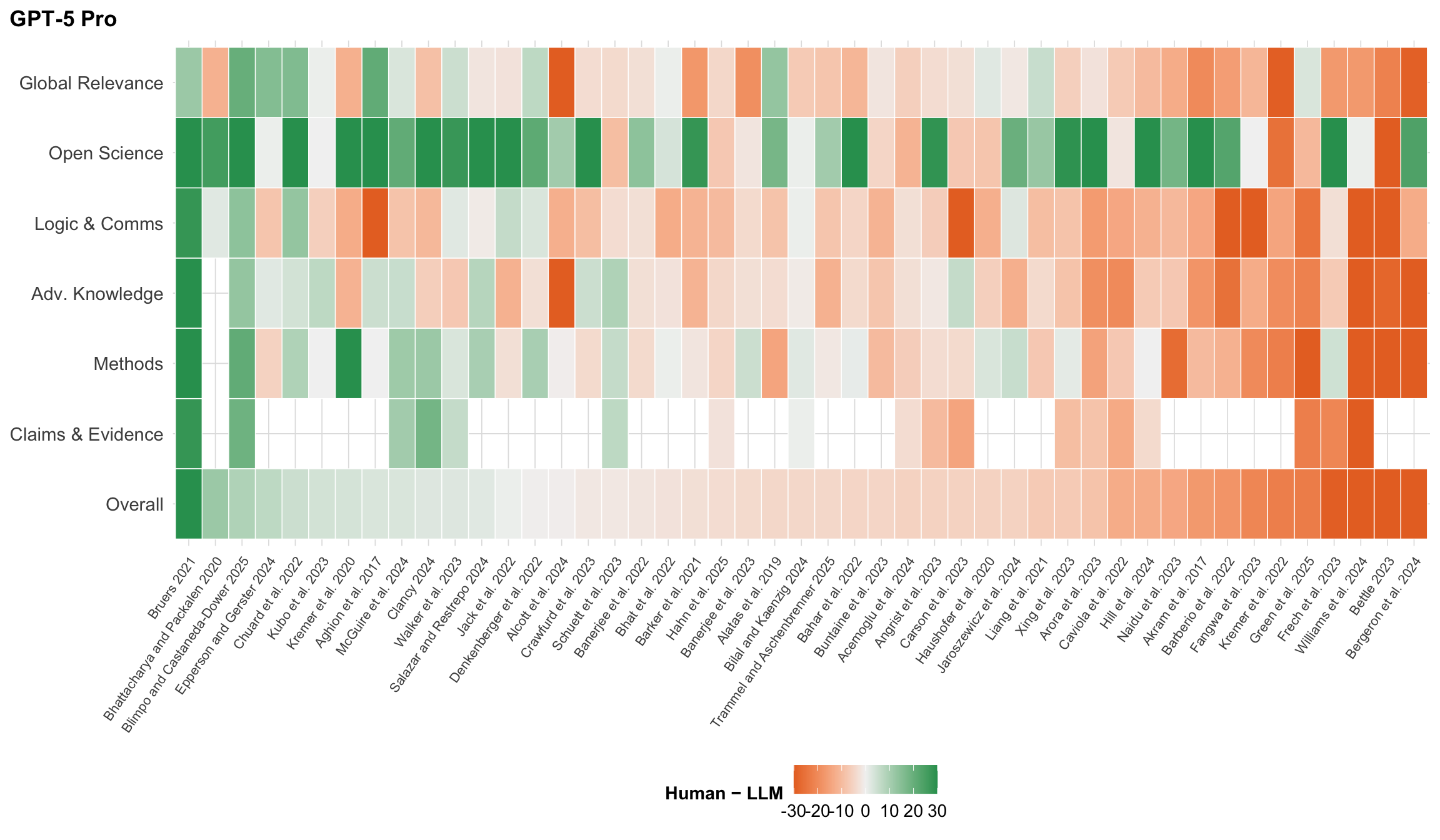
**Rating differences by paper and criterion.** @fig-gap-heatmap-main unpacks Human − GPT-5 Pro differences across all seven criteria simultaneously. Each column is a paper, each row a criterion, and tile colour encodes the signed difference (human mean minus GPT-5 Pro midpoint). Green tiles indicate the human panel rated the paper higher; orange tiles indicate GPT-5 Pro was more generous. Papers are sorted by overall difference.
```{r}
#| label: fig-gap-heatmap-main
#| fig-cap: "Human minus GPT-5 Pro rating difference for every paper (columns) and criterion (rows). Green tiles indicate the human mean was higher; orange tiles indicate GPT-5 Pro rated the paper higher. Colour is clamped to \u00b130 percentile points. Papers are sorted by overall difference."
#| fig-width: 12
#| fig-height: 7
#| code-fold: true
library("patchwork")

metric_order <- c("overall", "claims", "methods", "adv_knowledge",
                  "logic_comms", "open_sci", "gp_relevance")
metric_lab <- c(
  overall = "Overall",
  claims = "Claims & Evidence",
  methods = "Methods",
  adv_knowledge = "Adv. Knowledge",
  logic_comms = "Logic & Comms",
  open_sci = "Open Science",
  gp_relevance = "Global Relevance"
)

H_mean <- metrics_human |>
  filter(criteria %in% metric_order, paper %in% matched_papers) |>
  group_by(paper, criteria) |>
  summarise(h = mean(mid, na.rm = TRUE), .groups = "drop")

# Fixed paper order based on GPT-5 Pro overall difference
L_mean_primary <- llm_metrics |>
  filter(criteria %in% metric_order, model == primary_model, paper %in% matched_papers) |>
  group_by(paper, criteria) |>
  summarise(l = mean(midpoint, na.rm = TRUE), .groups = "drop")

Ddiff_primary <- inner_join(H_mean, L_mean_primary, by = c("paper", "criteria")) |>
  mutate(diff = h - l)

ord_p <- Ddiff_primary |>
  filter(criteria == "overall") |>
  arrange(desc(diff)) |>
  pull(paper)

build_gap_panel <- function(model_name, show_y_labels = TRUE,
                            llm_col = UJ_ORANGE) {
  L_mean_m <- llm_metrics |>
    filter(criteria %in% metric_order, model == model_name, paper %in% matched_papers) |>
    group_by(paper, criteria) |>
    summarise(l = mean(midpoint, na.rm = TRUE), .groups = "drop")

  Ddiff_m <- inner_join(H_mean, L_mean_m, by = c("paper", "criteria")) |>
    mutate(
      diff = h - l,
      crit = factor(criteria, levels = metric_order, labels = metric_lab[metric_order])
    )

  p <- ggplot(Ddiff_m, aes(x = factor(paper, levels = ord_p), y = crit, fill = diff)) +
    geom_tile(color = "white", linewidth = 0.25) +
    scale_fill_gradient2(
      low = llm_col, mid = "grey95", high = UJ_GREEN, midpoint = 0,
      name = "Human \u2212 LLM",
      limits = c(-30, 30),
      oob = scales::squish
    ) +
    labs(x = NULL, y = NULL, title = model_name) +
    theme_uj() +
    theme(
      axis.text.x = element_text(angle = 55, hjust = 1, vjust = 1, size = 8),
      panel.grid = element_blank()
    )

  if (show_y_labels) {
    p <- p + theme(axis.text.y = element_text(size = 11))
  } else {
    p <- p + theme(axis.text.y = element_blank())
  }

  p
}

if (length(ord_p) > 0) {
  build_gap_panel("GPT-5 Pro", show_y_labels = TRUE, llm_col = UJ_ORANGE) +
    theme(legend.position = "bottom")
} else {
  cat("Insufficient data for gap heatmap.\n")
}
```
Rows with uniformly green or orange tiles indicate papers where humans and GPT-5 Pro disagree systematically across all criteria, not just on one dimension. Columns with consistent colour suggest criteria-level biases---for instance, if "Open Science" is green across nearly all papers, humans may systematically reward data-sharing practices more than the model does. Multi-model comparisons in [Appendix A](results_ratings.qmd) reveal whether these disagreement patterns are GPT-5 Pro--specific or shared across frontier LLMs.
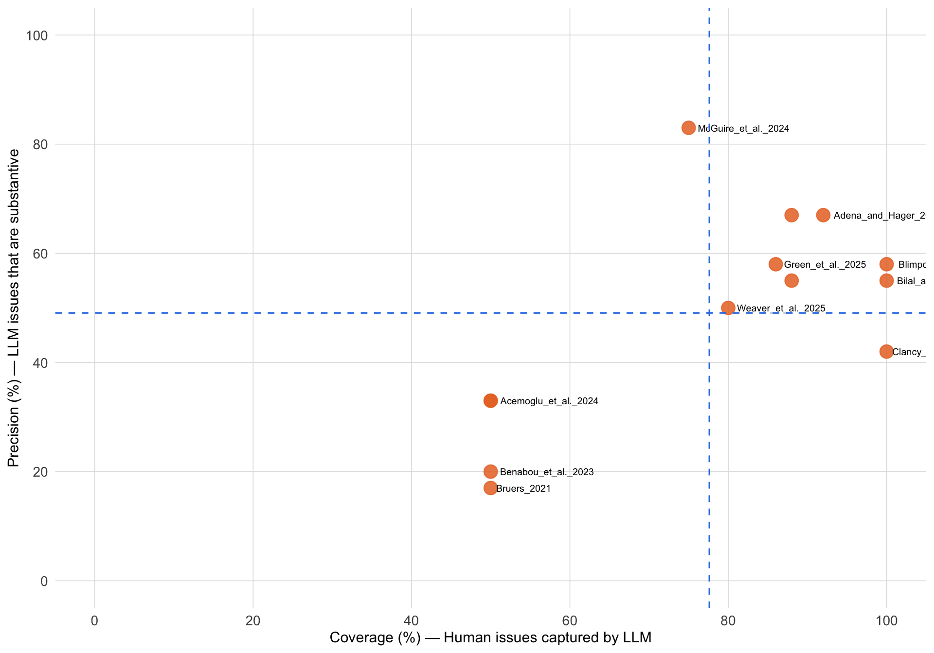
**Qualitative critique comparison.** Beyond numeric ratings, we compare the substantive critiques each model raises against the consensus issues identified by human experts. The figure below plots coverage---the fraction of human-identified concerns that the LLM also raised in some form---against precision---the fraction of LLM-raised issues that correspond to a substantive human concern. These metrics are assessed by GPT-5.2 Pro acting as an independent judge (see [Methods](methods.qmd) for the judging protocol). One of the 14 originally curated pairs (Peterman et al. 2025) is excluded: the judge flagged---and we verified against the paper---that the curated human critique belonged to a different manuscript, so results are reported for the remaining 13 pairs.
```{r}
#| label: load-critique-data
#| code-fold: true
#| code-summary: "Load critique comparison data"
#| message: false
comparison_results_file <- c(
  here("results", "key_issue_comp_results.json"),
  here("results", "key_issues_comparison_results.json")
)
comparison_results_file <- comparison_results_file[file.exists(comparison_results_file)][1]

has_critique_data <- FALSE

if (!is.na(comparison_results_file)) {
  comparison_file <- here("results", "key_issues_comparison.json")
  if (file.exists(comparison_file)) {
    comparison_data <- fromJSON(comparison_file)
    llm_results_raw <- fromJSON(comparison_results_file)
    llm_results <- llm_results_raw |>
      as_tibble() |>
      unnest_wider(comparison) |>
      select(
        gpt_paper,
        coverage_pct,
        precision_pct,
        any_of(c("matched_pairs", "unmatched_human", "unmatched_llm")),
        any_of(c("missed_issues", "extra_issues")),
        overall_rating,
        overall_justification,
        detailed_notes
      )
    comparison_data <- comparison_data |>
      left_join(llm_results, by = "gpt_paper")
    has_critique_data <- nrow(comparison_data) > 0 &&
      "coverage_pct" %in% names(comparison_data) &&
      any(!is.na(comparison_data$coverage_pct))
  }
}
```
```{r}
#| label: fig-coverage-precision-main
#| fig-cap: "Coverage (% of human-identified issues that the LLM also raised) vs Precision (% of LLM-raised issues that match a substantive human concern) for each paper, as assessed by GPT-5.2 Pro acting as judge. Dashed lines mark the cross-paper mean for each axis. Papers in the upper-right quadrant show strong alignment between human and LLM critiques."
#| fig-width: 10
#| fig-height: 7
if (has_critique_data) {
  crit_results <- comparison_data |>
    filter(!is.na(coverage_pct) & !is.na(precision_pct)) |>
    mutate(paper_short = str_trunc(gpt_paper, 25))

  ggplot(crit_results, aes(x = coverage_pct, y = precision_pct)) +
    geom_point(size = 4.5, color = UJ_ORANGE, alpha = 0.85) +
    geom_text(aes(label = paper_short), hjust = -0.1, vjust = 0.5, size = 2.6, check_overlap = TRUE) +
    geom_vline(xintercept = mean(crit_results$coverage_pct), linetype = "dashed", color = UJ_BLUE, linewidth = 0.6) +
    geom_hline(yintercept = mean(crit_results$precision_pct), linetype = "dashed", color = UJ_BLUE, linewidth = 0.6) +
    scale_x_continuous(limits = c(0, 100), breaks = seq(0, 100, 20)) +
    scale_y_continuous(limits = c(0, 100), breaks = seq(0, 100, 20)) +
    labs(
      x = "Coverage (%) \u2014 Human issues captured by LLM",
      y = "Precision (%) \u2014 LLM issues that are substantive"
    ) +
    theme_uj()
}
```
Coverage and precision vary substantially across papers. Averaged over the `r if (has_critique_data) sum(!is.na(comparison_data$coverage_pct))` focal papers, the model captures `r if (has_critique_data) sprintf("%.0f%%", mean(comparison_data$coverage_pct, na.rm = TRUE))` of human consensus issues (range `r if (has_critique_data) sprintf("%.0f--%.0f%%", min(comparison_data$coverage_pct, na.rm = TRUE), max(comparison_data$coverage_pct, na.rm = TRUE))`), while `r if (has_critique_data) sprintf("%.0f%%", mean(comparison_data$precision_pct, na.rm = TRUE))` of model-raised issues match a substantive human concern. Low precision partly reflects the reference set: the human consensus list contains only the issues evaluation managers prioritised, so model issues flagged by individual evaluators but not curated into the consensus count against precision. Because these metrics are themselves LLM-assessed, they should be interpreted with the caveat that an LLM judge may systematically over- or under-credit matches relative to a human annotator; the repository includes a browser-based annotation tool for manual validation of these alignment scores, which is ongoing.
Detailed paper-by-paper comparisons---including matched issue pairs with severity labels, structural difference tables, and per-evaluator breakdowns---appear in [Appendix B: Critiques & Key Issues](results_critiques.qmd). Extended quantitative analysis including all six models, per-criterion correlations, bootstrap confidence intervals, tier prediction accuracy, and cost-quality trade-offs is reported in [Appendix A: Results Ratings](results_ratings.qmd). The full LLM reasoning traces and assessment summaries are available in [Appendix C: LLM Traces](appendix_llm_traces.qmd).
**Agreement summary.** @tbl-model-agreement-main shows GPT-5 Pro's agreement split into a **primary matched group** (same `r hh_n` papers as the H–H baseline, enabling like-for-like comparison) and a **secondary full-sample group** (all `r n_focal` matched papers). In the Spearman *ρ* column, the H–H row shows individual-vs-individual *ρ* (the reference, already on the natural scale); GPT-5 Pro rows show *ρ* vs. the human mean, which is upward-biased. The **ρ adj.** column applies the Spearman-Brown correction to GPT-5 Pro rows only, making them directly comparable to H–H *ρ*. Six-model comparison in [Appendix A, Table A2](results_ratings.qmd#tbl-agreement).
```{r}
#| label: tbl-model-agreement-main
#| tbl-cap: !expr cap_tbl_model_agreement
#| code-fold: true
model_compare_data <- llm_metrics |>
  filter(criteria == "overall", model == "GPT-5 Pro", paper %in% focal_papers) |>
  left_join(
    human_avg |> select(paper, human_mid),
    by = "paper"
  ) |>
  filter(!is.na(human_mid))

if (nrow(model_compare_data) > 0) {

  # Matched sample: same papers used for H-H baseline (≥2 human raters)
  lfl_papers_main  <- hh_pairs$paper
  model_lfl        <- model_compare_data |> filter(paper %in% lfl_papers_main)
  raw_rho_lfl      <- cor(model_lfl$human_mid, model_lfl$midpoint,
                          method = "spearman", use = "complete.obs")
  n_lfl            <- nrow(model_lfl)

  # Full sample: all focal papers
  raw_rho_full <- cor(model_compare_data$human_mid, model_compare_data$midpoint,
                      method = "spearman", use = "complete.obs")
  n_gpt        <- nrow(model_compare_data)

  make_gpt_row <- function(data, rho, n_papers, label = "GPT-5 Pro") {
    tibble(
      Model          = label,
      N              = n_papers,
      `Spearman ρ` = sprintf("%.3f", rho),
      `ρ adj.`  = sprintf("%.3f", rho * sb_factor),
      `95% CI`       = spearman_ci95(rho, n_papers),
      `Pearson r`    = round(cor(data$human_mid, data$midpoint, use = "complete.obs"), 3),
      `Mean bias`    = sprintf("%+.1f", mean(data$midpoint - data$human_mid, na.rm = TRUE)),
      MAE            = sprintf("%.1f", mean(abs(data$midpoint - data$human_mid), na.rm = TRUE))
    )
  }

  hh_row_main <- tibble(
    Model          = "Human-Human",
    N              = hh_n,
    `Spearman ρ` = sprintf("%.3f", hh_spearman),
    `ρ adj.`  = "-",
    `95% CI`       = spearman_ci95(hh_spearman, hh_n),
    `Pearson r`    = round(hh_pearson, 3),
    `Mean bias`    = hh_bias,
    MAE            = sprintf("%.1f", hh_mae)
  )

  gpt_matched_row <- make_gpt_row(model_lfl, raw_rho_lfl, n_lfl)
  gpt_full_row    <- make_gpt_row(model_compare_data, raw_rho_full, n_gpt)

  model_compare_tbl <- bind_rows(hh_row_main, gpt_matched_row, gpt_full_row)

  knitr::kable(model_compare_tbl,
               align    = c("l", rep("r", ncol(model_compare_tbl) - 1)),
               booktabs = TRUE) |>
    kableExtra::row_spec(1, bold = TRUE, background = "#f0f8f0") |>
    kableExtra::pack_rows(
      sprintf("Matched sample: same %d papers as H-H baseline (primary)", hh_n),
      1, 2, bold = TRUE, italic = FALSE, color = "black"
    ) |>
    kableExtra::pack_rows(
      sprintf("Full sample: all %d GPT-5 Pro matched papers (secondary)", n_gpt),
      3, 3, bold = FALSE, italic = TRUE
    )
}
```
The Fisher-z intervals in @tbl-model-agreement-main quantify uncertainty in each correlation separately; to make an uncertainty statement about the *comparison itself* we add a paired bootstrap over papers (2,000 resamples of the `r hh_n` matched-group papers). Each draw recomputes the GPT-5 Pro--human-mean rank correlation, applies that draw's own Spearman-Brown correction, and takes the difference against the human--human pairwise correlation on the same draw. The resulting distribution of the adjusted difference (ρ adj. − ρ~HH~) spans `r fmt_ci(boot_ci_diff)`: the interval includes zero, so at this sample size we cannot statistically separate the model from an additional human rater---the two correlations are comparable, not demonstrably ordered. This is the precise sense in which GPT-5 Pro "performs within the human inter-rater range."
@tbl-criteria-agreement-main breaks the same agreement metrics down by evaluation criterion for GPT-5 Pro. The **H-H ρ** column shows pairwise human-human Spearman ρ for each criterion as a reference — note that raw LLM ρ is upward-biased relative to H-H ρ by the mean-vs-individual asymmetry (see @tbl-model-agreement-main). Criteria where H-H ρ is itself low indicate genuine expert disagreement; low LLM agreement on those criteria is therefore expected rather than a model failure.
```{r}
#| label: tbl-criteria-agreement-main
#| tbl-cap: !expr cap_tbl_criteria_agreement
#| code-fold: true
criteria_order <- c("overall", "claims", "methods", "adv_knowledge",
                    "logic_comms", "open_sci", "gp_relevance")
criteria_labels <- c(
  overall      = "Overall",
  claims       = "Claims & Evidence",
  methods      = "Methods",
  adv_knowledge = "Adv. Knowledge",
  logic_comms  = "Logic & Comms",
  open_sci     = "Open Science",
  gp_relevance = "Global Relevance"
)

# Human-human pairwise Spearman rho per criterion (ceiling reference)
hh_crit_pairs <- metrics_human |>
  filter(criteria %in% criteria_order, paper %in% focal_papers) |>
  select(paper, criteria, evaluator, mid) |>
  distinct() |>
  group_by(paper, criteria) |>
  filter(n() >= 2) |>
  mutate(slot = paste0("E", row_number())) |>
  ungroup() |>
  pivot_wider(names_from = slot, values_from = c(mid, evaluator)) |>
  filter(!is.na(mid_E1), !is.na(mid_E2))

hh_crit_rho <- hh_crit_pairs |>
  group_by(criteria) |>
  summarise(
    `H-H ρ` = round(cor(mid_E1, mid_E2, method = "spearman", use = "complete.obs"), 3),
    .groups = "drop"
  )

human_by_crit <- metrics_human |>
  filter(criteria %in% criteria_order, paper %in% focal_papers) |>
  group_by(paper, criteria) |>
  summarise(human_mid = mean(mid, na.rm = TRUE), .groups = "drop")

crit_compare_data <- llm_metrics |>
  filter(criteria %in% criteria_order, model == "GPT-5 Pro", paper %in% focal_papers) |>
  inner_join(human_by_crit, by = c("paper", "criteria"))

if (nrow(crit_compare_data) > 0) {
  crit_tbl <- crit_compare_data |>
    group_by(criteria) |>
    summarise(
      `Spearman ρ` = round(cor(human_mid, midpoint, method = "spearman",
                                    use = "complete.obs"), 3),
      `Pearson r`  = round(cor(human_mid, midpoint, use = "complete.obs"), 3),
      `Mean bias`       = sprintf("%+.1f", mean(midpoint - human_mid, na.rm = TRUE)),
      RMSE              = round(sqrt(mean((midpoint - human_mid)^2, na.rm = TRUE)), 1),
      .groups = "drop"
    ) |>
    left_join(hh_crit_rho, by = "criteria") |>
    mutate(Criterion = factor(criteria, levels = criteria_order,
                              labels = criteria_labels[criteria_order])) |>
    select(Criterion, `H-H ρ`, `Spearman ρ`, `Pearson r`, `Mean bias`, RMSE) |>
    arrange(Criterion)

  knitr::kable(crit_tbl, align = c("l", rep("r", 5))) |>
    kableExtra::column_spec(2, bold = TRUE)
}
```
**Journal-tier predictions and verifiable outcomes.** Beyond percentile ratings, both evaluator types predict where each paper *will* publish on The Unjournal's 0--5 journal-tier scale. Unlike percentile scores, these predictions eventually resolve against an observable outcome: the venue where the paper actually publishes.
```{r}
#| label: compute-tier-outcomes
#| include: false
# Realized publication tier from The Unjournal's recorded publication status.
# Mapping is deliberately coarse and conservative; ambiguous entries
# ("? journal", "uncertain peer review"), R&R/forthcoming/conditionally
# accepted, and book chapters are treated as unresolved.
tier_outcomes <- research |>
distinct(label_paper, publication_status) |>
filter(!is.na(label_paper)) |>
mutate(
status_l = str_to_lower(coalesce(publication_status, "")),
realized_tier = case_when(
str_detect(status_l, "~top journal") ~ 4.5,
str_detect(status_l, "decent journal") ~ 3.0,
str_detect(status_l, "psychology journal") ~ 2.5,
TRUE ~ NA_real_
)
)
human_tier_will <- rsx_research |>
filter(criteria == "journal_predict") |>
mutate(mid = suppressWarnings(as.numeric(middle_rating))) |>
filter(!is.na(mid), !is.na(label_paper)) |>
distinct(label_paper, evaluator, mid) |>
group_by(paper = label_paper) |>
summarise(human_will = mean(mid), .groups = "drop")
gpt_tier_will <- llm_tiers |>
filter(model == "GPT-5 Pro", tier_kind == "tier_will") |>
distinct(paper, .keep_all = TRUE) |>
select(paper, gpt_will = score)
tier_df <- human_tier_will |>
inner_join(gpt_tier_will, by = "paper") |>
left_join(tier_outcomes |> select(paper = label_paper, publication_status, realized_tier),
by = "paper")
n_tier_pred <- nrow(tier_df)
tier_pred_rho <- cor(tier_df$human_will, tier_df$gpt_will, method = "spearman")
tier_resolved <- tier_df |> filter(!is.na(realized_tier)) |> arrange(desc(realized_tier))
n_tier_resolved <- nrow(tier_resolved)
n_tier_open <- n_tier_pred - n_tier_resolved
tier_mae_human <- mean(abs(tier_resolved$human_will - tier_resolved$realized_tier))
tier_mae_gpt <- mean(abs(tier_resolved$gpt_will - tier_resolved$realized_tier))
```
Human and GPT-5 Pro tier predictions agree at Spearman ρ = `r sprintf("%.2f", tier_pred_rho)` (N = `r n_tier_pred` papers with both predictions)---stronger agreement than on any percentile criterion, suggesting that "where will this publish" is a better-anchored question than "what percentile is this paper." For `r n_tier_resolved` of these papers, The Unjournal's records already show a resolved publication outcome that we can map to the tier scale (@tbl-tier-outcomes). On this small resolved set, mean absolute error against the realized tier is `r sprintf("%.2f", tier_mae_gpt)` tiers for GPT-5 Pro and `r sprintf("%.2f", tier_mae_human)` for the human panel mean---both track outcomes to within roughly two-thirds of a tier, and the sample is far too small to rank the two.
```{r}
#| label: tbl-tier-outcomes
#| tbl-cap: "Papers with resolved publication outcomes: predicted vs realized journal tier (0--5 scale). Realized tier maps The Unjournal's recorded publication status: '~top journal' = 4.5, 'decent journal' = 3.0, field journal = 2.5. Ambiguous statuses, R&R/forthcoming, and book chapters are treated as unresolved and excluded. Human prediction is the evaluator mean."
#| code-fold: true
if (n_tier_resolved > 0) {
  tier_resolved |>
    transmute(
      Paper = paper,
      `Recorded outcome` = publication_status,
      `Realized tier` = realized_tier,
      `Human prediction` = round(human_will, 2),
      `GPT-5 Pro prediction` = round(gpt_will, 2)
    ) |>
    knitr::kable(align = c("l", "l", rep("r", 3)))
}
```
Two caveats apply. First, most of these papers were published before the model's training cutoff, so GPT-5 Pro may partly *recall* venues rather than predict them; human predictions were made before the publication outcome was known, which makes this comparison structurally generous to the model. Second, the remaining `r n_tier_open` papers with registered predictions from both evaluator types are still unresolved (working papers, R&R, or forthcoming). These predictions are locked in this repository and can be scored as outcomes accrue---a prospective validation design that sidesteps the contamination concern entirely, since future publication decisions cannot appear in any current model's training data.
::: {.content-visible when-format="pdf"}
All appendices, interactive figures, and full code are available at the companion website: <https://llm-uj-research-eval.netlify.app>. Source code and data are hosted at <https://github.com/valentinklotzbuecher/llm-uj-research-eval>.
:::